REM-RAM

Featured

REMRAM: An Introduction.

Hello World! An apt beginning to a blog which I hope will (eventually!) have a fair amount of quasi-compsci and quasi-math content. To be honest, I hope it will be quasi-everything, from neuroscience to mathematics, artificial intelligence to linguistics. The unifying theme: to reveal some of the hidden connecting threads on which the observable world sits.

But I am getting ahead of myself already.

Perhaps I should have started by explaining the blog title. REMRAM, quite possibly one of the worst ideas to emerge from the complex system of neurons unfortunate enough to inhabit my brain. I am tempted to defer to the illusory nature of free-will and claim I never really had any choice in the matter to begin with. I won’t though.

REM Rapid eye movement sleep (REM sleep or REMS) is a unique phase of sleep in mammals and birds, distinguishable by random/rapid movement of the eyes, accompanied with low muscle tone throughout the body, and the propensity of the sleeper to dream vividly.

RAM Random-access memory (RAM /ræm/) is a form of computer memory that can be read and changed in any order, typically used to store working data and machine code. A random-access memory device allows data items to be read or written in almost the same amount of time irrespective of the physical location of data inside the memory.

Thanks Wikipedia! So by combining the words REM and RAM, I hope to combine the dream world and the world of memory. Creating a working memory of different subjects that interest me whilst peering through the looking-glass and unveiling the phantasmagoria behind them all. The fact that these acronyms come from the two rapidly converging spheres of brains and machines respectively (which will be amongst my main focuses) an added bonus. I leave you with a parting question, do androids dream of electric sheep?

ENTROPY: Communication, Disorder and Perpetual Motion Machines.

As promised, an article on the fascinating concept of Entropy. A real go-getter, entropy seems to have it’s hands in a million different pies (probably because it knows the pies will inevitably become a massive pile of sloppy, mushy, disorder and who would want to eat that?). If you didn’t get that joke, hopefully you will by the end. Let me take you by the hand, and lead you through entropy land.

HEALTH WARNING: feel free to skip over any/all math formulae, just imagine they are not there.

Decision Trees

A decision tree is a machine learning algorithm which tries to find the most efficient tests to make a prediction. For example, given information about tumours (height, volume, colour, growth rate etc.) the decision tree learns the questions it should ask to determine whether the tumour is malignant. So how does it identify these tests?

As I mentioned in my article on Lorenz Curves https://remramryan.home.blog/2019/12/16/lorenz-curves-measuring-inequality/ Gini Index (GI) is one measure used in Decision Tree algorithms. This is because GI measures the inequality within a set of data. Decision Tree algorithms leverage this in order to segment the data space into sub-sections, which have lower inequality (they are more equal).

A decision tree, illustrating our intuition that geographical location is highly correlated with gdp. We can pretty much determine a European Country’s location 3 questions about GDP/ Capita. Although some important misclassifcations are Poland as western, Romanian as Southern which are understandable.

An alternative metric for calculating homogeneity of subspaces would be Entropy, as used in the above example. Defined as: $H(x) = - \sum_{i=1}^m p(x_i)log(p(x_i))$
Where, given an observation $x$ is taken from the subspace, and $m$ possible ‘categories’ $x_1, x_2, ... , x_m$ , $p(x_i)$ is the probability observation $x$ is of type $x_i$ .

To understand how this expression captures the relative homogeneity, or conversely, disorder, consider the case with only two possible states. Now we have
$H(p) = - plogp - (1-p)log(1-p)$ . So plotting $H$ as a function of $p$ we get:

Entropy diagram for a state space of size 2.

In this example, a 50-50 mix of the two different states results in a maximum entropy, whereas if we have perfect homogeneity the entropy is 0. Right, so entropy measures disorder, but why does this function work? To understand this, we will need to take a quick dive into Information Theory.

Information Theory

Step up Claude Elwood Shannon, the (God)Father of Information Theory. We will pick up his story from WWII, where Shannon was heavily involved in studying cryptographic systems. During this time, Shannon came in to contact with Alan Turing the (God)Father of AI (and computing in general). His work on cryptographic systems and Alan Turing’s influence, led Shannon to the creation* of Information Theory. Shannon also had many other hobbies, including inventing the first wearable computer which was designed for cheating at roulette. What a guy.

*Is mathematics created or discovered, I hope to write on this at some point in the future.

So Information Theory, what is it? Information theory studies the quantification, storage, and communication of information. – Wikipedia. Pretty intuitive, yet not very insightful. Well the fundamental quantity studied in Information Theory is, you guessed it, entropy. However, we can define a quantity called Information (content), to which entropy is intrinsically related. Let $X$ be a random variable with probability mass function $p$ , then $I(x) = -logp(x)$ . Can you now guess the relationship between entropy and information? $H(X) = \mathbb{E} [I(X)]$ Entropy, is the average information gained after observing a random variable.

Information tells us the number of bits gained when we observe a random variable. For instance, the information $I(H)$ of $X$ where $X$ is a fair coin, is 1. (Or tautologically, observing a bit as being 1, carries 1 bit of information — this is in fact how bits are defined!). Therefore entropy gives us the expected information gain after observing a random variable.

To gain a more intuitive feel as to why (Shannon) entropy is fundamental, consider this experiment measuring the communication potential of ants. http://reznikova.net/R-R-entropy-09.pdf. They estimate that ants can transfer ~1 bit of information per minute (the investigation involves starving ants and placing food at exactly one leaf of a binary tree). So entropy tells us something about the amount of information that could be contained in a given message. For the interested reader: Shannon showed that Entropy can be defined axiomatically. (The entropy function, is the unique function fitting a few desired axioms).

Alright it is now time to change lanes. If you had heard the word entropy before, it was most likely in relation to the fabled second law of thermodynamics. You may be wondering, are they related, are they the same, what is the connection?

The Second Law of Thermodynamics

Let us start with a definition. The second law of thermodynamics states that the total entropy of an isolated system can never decrease over time, and is constant if and only if all processes are reversible. Isolated systems spontaneously evolve towards thermodynamic equilibrium, the state with maximum entropy. — Wikipedia. Or in English: Ordered things will tend towards disorder. For example, ice melts. $H_2 O$ molecules in ice have more ‘order’ than they do in water. The second law of thermodynamics states that this change is inevitable (given we are working in an isolated system). Basically, everything we know and love will eventually turn to mush, harrowing stuff.

For an intuitive notion of why this is true. Consider the following thought experiment. There is a box containing a gas. However, all the gas particles are situated in the upper left hand corner of the box (highly ordered). Over time, clearly the gas will spread out to fill the box (solely due to probability) and thus entropy (disorder) will increase.

The particles naturally spread out, from a state of low entropy to a state of high entropy.

Here entropy is defined over possible (micro)states of particles in the box. $H = -k_b \sum_{i} p_i log(p_i)$ . Where $k_b$ is the Boltzmann constant and $p_i$ is the probability of the system being in microstate $i$ . Looks familiar right. Here is the awaited connection, this thermodynamic entropy (under certain conditions) is simply the number of Shannon bits needed to define the microstate of a system, given it’s macrostate (temperature, energy, number of particles etc.). Or as put by G. N. Lewis in 1930, ‘Gain in Entropy means loss of information, and nothing more’.

Perpetual Motion: Knowledge is Power

One consequence of the second law of thermodynamics was to render impossible attempts to build a ‘perpetual motion’ machine. A perpetual machine is something that can simply power itself, with no need of any energy source. A perpetual motion machine would effectively solve the climate crisis by generating power. Sound too good to be true? Well, as you know such a machine is not possible. If it were, we could place the machine in our example box from earlier, using it to force the gas molecules to stay in the upper left-hand corner. This would violate the second law of thermodynamics, thus the machine cannot have existed. But if entropy is information, couldn’t we use information to power our perpetual motion machine? Bring on the Szilard engine!

The Szilard engine is a box, with two compartments separated by a sliding wall . Lets keep things simple and imagine there is just a single particle in the box. Suppose we knew which compartment the particle was in, which is exactly 1 Shannon bit of information (see the coin flip example from earlier). Well then the pressure in this side of the box will force the sliding wall to the opposite side, thus doing work. Crucially because we knew which way the wall would be forced to slide, we can set up a pulley with a weight and lift that weight, using the work done by the sliding wall. So knowledge really is power!

It would be remiss of me, to say this was not controversial. The necessity of knowledge for Szilard’s engine to function is debated, and its discussion preempts the discussions of measurement in quantum mechanics. However these engines certainly exist, see https://www.pnas.org/content/pnas/111/38/13786.full.pdf.

Okay, I feel like that is enough for today. There is, however, much much more to talk about! From the arrow of time, to black holes, to the Heisenberg principle of quantum mechanics, entropy is everywhere. Hopefully I will get round to discussing these in a follow up post, before those pies sink into soggy disorder that is!

LORENZ CURVES: Measuring Inequality.

Recently, my sister asked the best way to produce some illustrative Lorenz curves for an essay she was writing. Now, I had heard of Lorenz curves but I had no idea what they actually were. Buckle-up for our first mathematical adventure!

Enter Max O. Lorenz, creator of the Lorenz curve, mostly interested in railways and such. Whilst, railways are surely interesting, and perhaps they were more interesting in the 1910s, Lorenz’s most obvious legacy is the curve bearing his name. The Lorenz curve allows us to picture ‘clearly in our minds the relative distribution of wealth’ according to Willford I. King – who originally coined the term.

The ‘First’ Lorenz Curve

So what is a Lorenz Curve you ask? We’ll come back to that later. (I did warn you this was an adventure). Let’s start with a seemingly unrelated problem from statistics.

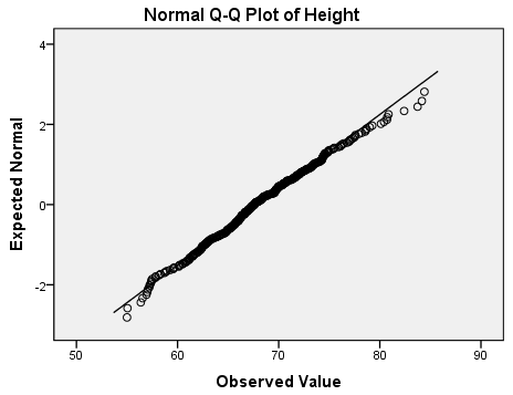
Say I gave you the heights of a 100 people and asked you to verify that the heights came from a normal distribution, what would you do?

YOU: Easy! A student t-test!
ME: *rolls eyes* Sure, fine, yeah that’s true you could do that. How about a more visual way?
YOU: Easy! Plot a histogram!
ME: *sigh* Well yes, you could definitely do that. But how would you know the distribution was definitely normal?
YOU: No clue mate.
ME: *rubs hands* Well my friend, let me introduce you to the QQ plot.

Quantile-Quantile plots

The quantile-quantile plot is pretty much what it says on the tin. Given a theoretical distribution we can calculate quantiles. You are already very familiar with quantiles. For example, you are in the bottom decile for height, you are in the smallest 10% of people in the given population. If exactly 10% of people are under 150cm, then 150cm is the 10th quantile. Now if a good model for height is a normal distribution and we calculate the quantiles for both the normal distribution, $N_i$ and the empirical data $H_i$ , what will happen if we plot the points $(H_i, N_i)$ ?

Wala! The points lie on a roughly straight line? This is because we have the same shapes for the observed and empirical distributions. (Hopefully this will be clear with a bit of thought).

Right so what was that you said about wealth inequality?

Lorenz Curves

It turns out the Lorenz curve is simply a special case of a qq plot. We still calculate the quantiles of the empirical distribution as before, however, this time we plot them against the quantiles from a uniform distribution. I.e. we plot the quantiles $H_i$ at regularly spaced intervals.

An example of a Lorenz curve where the wealth distribution was generated from a pareto distribution.

Why, then, are these curves so popular? If you’ve ever heard a politician (R.I.P. Jeremy Corbyn) mention something like, 10% of people in the U.K. own 40% of its wealth (real statistic btw), then you will know how powerful it is. Each point on this curve reads exactly that statistic. So with Lorenz Curves it is incredibly easy to visually compare different wealth distributions on the same scale. Given this, you may naturally wonder if this graph can give us a general statistic for inequality, the answer is yes!

The Gini in a Bottle

I first came across the Gini Coefficient when studying decision trees. A supervised machine learning algorithm designed to classify data. But before we get into that, another digression, this time into ROC (reciever operating characteristic) curves.

The receiver operating characteristic, widely used in Machine Learning for binary classification has a very interesting history:

The ROC curve was first used during World War II for the analysis of radar signals before it was employed in signal detection theory. Following the attack on Pearl Harbor in 1941, the United States army began new research to increase the prediction of correctly detected Japanese aircraft from their radar signals. For these purposes they measured the ability of a radar receiver operator to make these important distinctions, which was called the Receiver Operating Characteristic. – Wikipedia

More recently the ROC is used to compare different binary classifications, with a key metric being the Area Under the Curve (AUC). The ROC is the plot of the True Positive Rate (TPR or sensitivity/recall) against the False Positive Rate (FPR or 1 – specificity) whilst varying the classification threshold. Or using the terminology of hypothesis testing, the ‘power’ against ‘type 1 error’. Phew, why do we have so many terms for the same quantity?

So what does the AUC represent? The AUC is the probability a classifier will rank a randomly chosen positive instance higher than a randomly chosen negative one. So AUC can be used as a general metric for comparing binary classifiers (a score of 1, would be a perfect classifier). Alright so how could all this possibly be related to Lorenz Curves? To answer this, lets finally define the Gini Coefficient.

The gini coefficient is defined as twice the area between the Lorenz Curve and the straight line. A high Gini score (the highest clearly being 1) represents a very unequal wealth distribution (the richest person has all the wealth).

A very surprising glimpse of the gini indices over time

Now, it turns out that the ROC curve is the inverse of the Lorenz curve, and thus the gini coefficient is extremely closely related to the AUC score, $2AUC - 1 = GINI$ . So given this new perspective, we can think of the Lorenz curve as implicitly encoding the probability an individual is wealthier than they should be (if you think wealth should be distributed completely equally of course).

To go further down the rabbit hole, see my post on Entropy. Can you separate the wood from the Decision Trees?